You know those people who say things to the effect of, “One in two people has below average intelligence,” with a really smug look on their face? The satisfaction they seem to get from flaunting their fundamental misunderstanding of statistics makes it pretty clear which side of average their intelligence falls on.
Well, you either clicked a “read more” link, or you’re reading a full-text RSS feed. Either way, I can talk about statistics now. First of all, let’s establish what an average actually is. The average, or mean, is defined as the sum of all values divided by the number of values. It’s important to remember that outliers can have a big effect on the mean. The median is the value with an equal number of values on either side of it, but that’s a different concept. Here are some nice probability density functions:
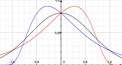
You’ve almost definitely seen the black curve before: it’s the so-called normal distribution, often called the bell curve. It’s nice and symmetrical. If a data set follows this distribution, a randomly selected value will be equally likely to be negative or positive (median of zero), and if you sum all the values and divide by the number of values, you’ll get zero (mean of zero).
The other two curves are skew-normal distributions. The red curve has left skew (κ = ½), and the blue curve has right skew (κ = −½). Both of these distributions still have a median of zero — with either of these distributions, a randomly selected value from a large data set is equally likely to be positive or negative.
But look at the way they trail away to one side. Take the red curve — it stops rather abruptly on the right, but trails away off to the left. These values bring the mean down. The mean is less than zero for the left-skewed distribution, and greater than zero for the right-skewed distribution. A randomly selected value is more likely to be higher than the mean for the left-skewed distribution, and more likely to be lower than the mean for the right-skewed distribution. Less than half the values are below average for the red distribution, and more than half are below average for the blue distribution. (The actual values of the means of these distributions are about −0.266 and 0.266 respectively.)
If that seems a bit abstract, we can make examples with small sets of real numbers, too. For our first data set, let’s use {1, 3, 5, 7, 9}. The statistics are pretty easy on this: sum of 25, mean of 5 and median of 5. The average is 5, and a randomly selected value is equally likely to be on either side of 5. The data has no skew.
Now let’s try a left-skewed data set: {1, 2, 5, 6, 6}. The sum is 20, the mean is 4 and the median is 5. A randomly selected value is clearly more likely to be greater than the average: there are three values greater than 4, compared to two values that are less. The values are still evenly distributed around the median.
(A right-skewed data set with equivalent characteristics is {4, 4, 5, 8, 9} — you can work through it yourself if you want to see how it goes.)